Food Web Plots with webplotviz

library(rpathviz)
library(Rpath)

Overview

webplotviz() creates a static food web diagram from an Rpath object. Nodes represent functional groups and fleets; node size reflects biomass and edges represent predator–prey interactions and fishing pressure. The y-axis is fixed to trophic level.

Basic usage — Anchovy Bay

AB.params is a small fictional ecosystem included in the Rpath package. It is a good starting point because it renders quickly.

# Build the Rpath balanced model
Rpath.obj <- rpath(AB.params, eco.name = "Anchovy Bay")

# Plot with default settings
webplotviz(Rpath.obj)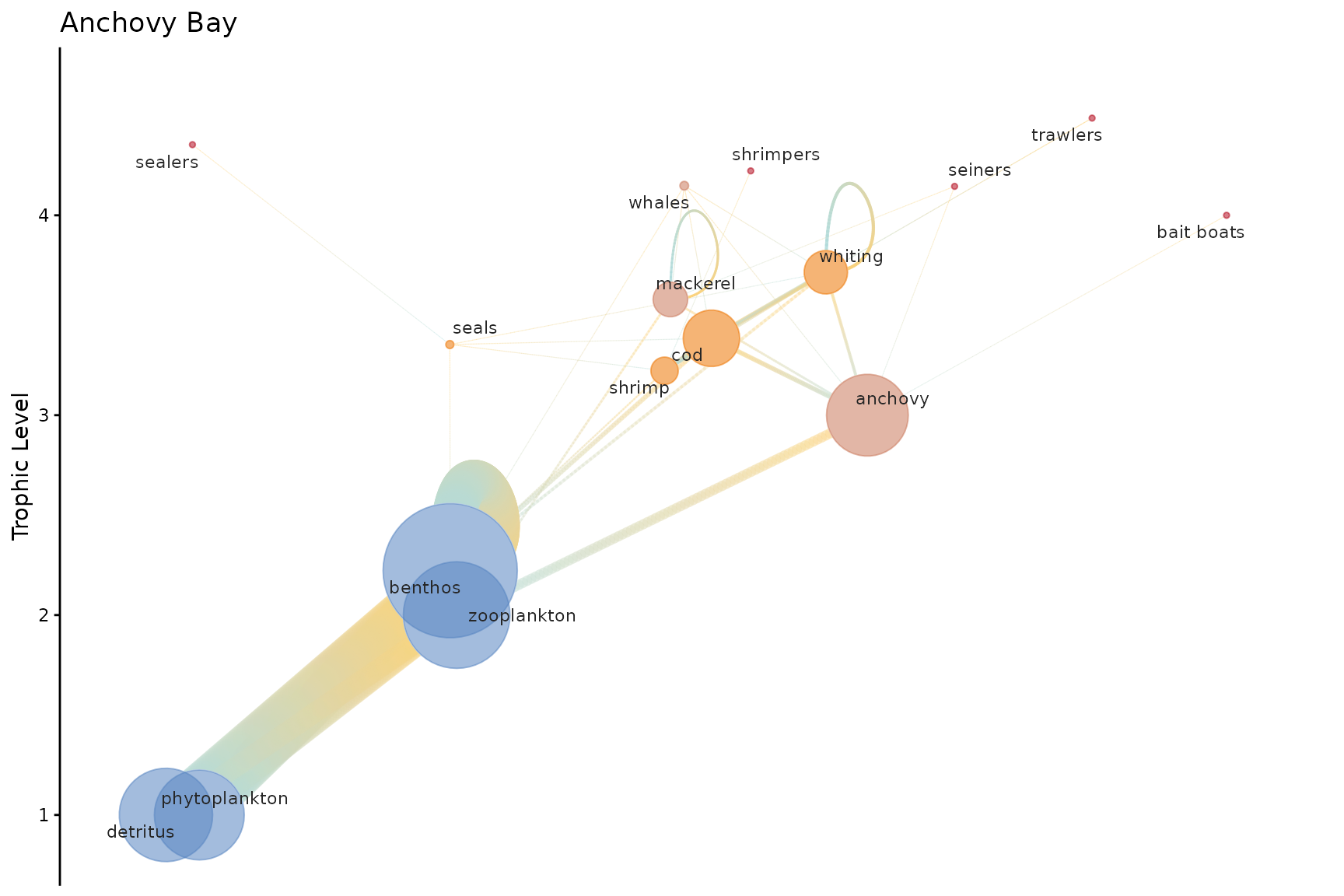

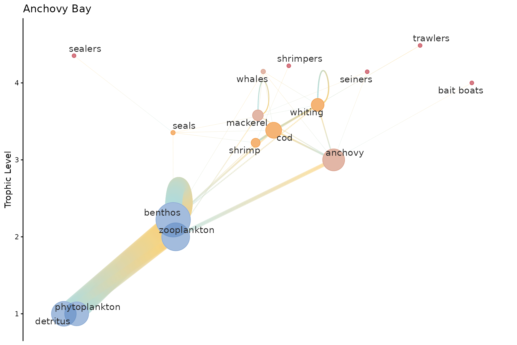
Customizing node size and spacing

Use h_spacing to spread nodes horizontally and node_size_min / node_size_max to control the range of node sizes.

webplotviz(
  Rpath.obj,
  h_spacing     = 5,
  node_size_min = 2,
  node_size_max = 20,
  text_size     = 4
)

Changing color palettes

Two built-in palettes are available: "rpath_pal_dark" (default) and "rpath_pal_light". You can also supply a custom vector of hex colors.

webplotviz(Rpath.obj, groups_palette = "rpath_pal_light")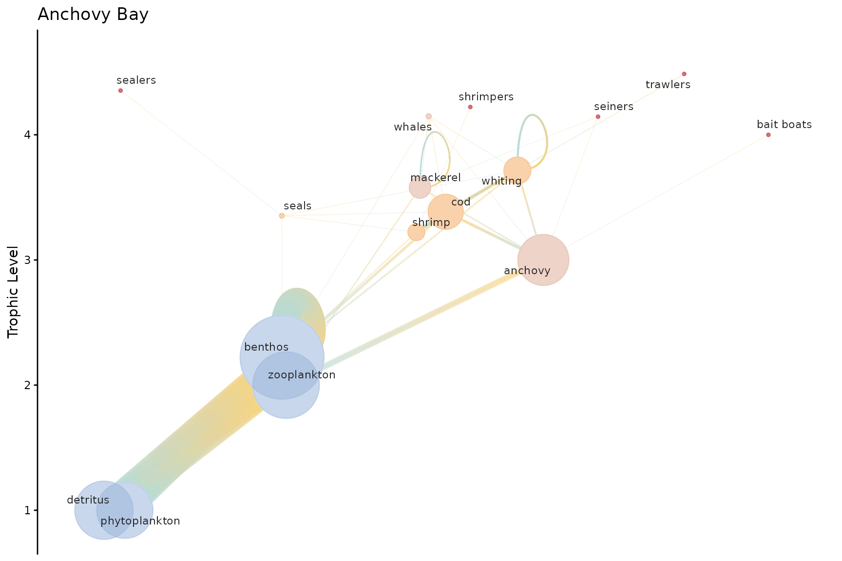

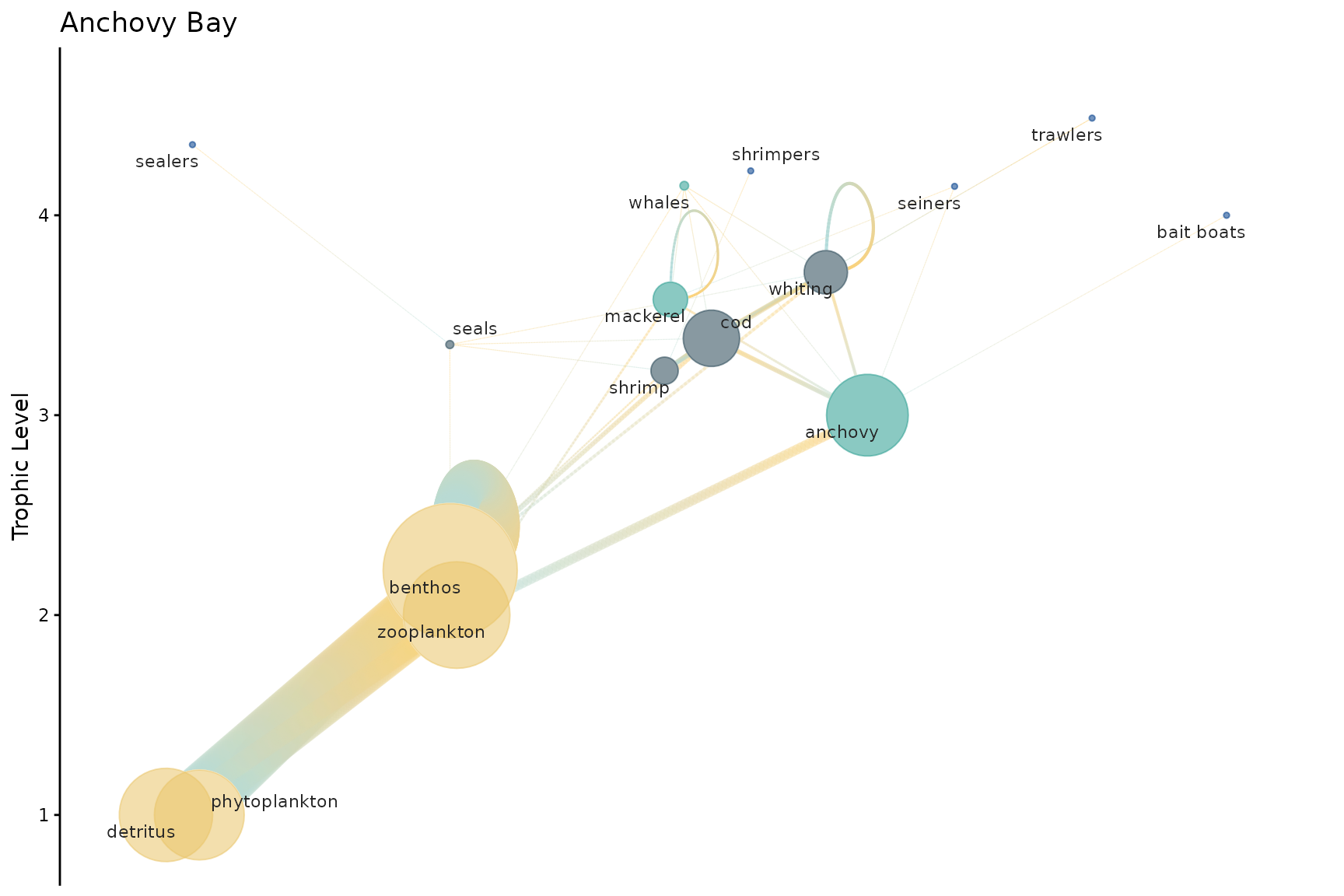
webplotviz(
  Rpath.obj,
  groups_palette = c("#264653", "#2a9d8f", "#e9c46a", "#f4a261", "#e76f51"),
  fleet_color    = "#023e8a"
)

Rendering options — `labels` and `gradient`

Two parameters control the visual style and rendering speed of the plot.

labels (default TRUE) draws group name labels using ggrepel to avoid overlap. Label placement is the largest single rendering cost — on a 54-group model it accounts for roughly half the total render time. Set labels = FALSE when you want a fast preview or a clean export that you’ll annotate separately.

gradient (default FALSE) draws each edge with a prey-to-predator colour gradient instead of a fixed line.col colour. It adds a visual cue for interaction direction but has a modest render cost.

# labels = FALSE: fastest render, useful for large-web previews
webplotviz(Rpath.obj, labels = FALSE)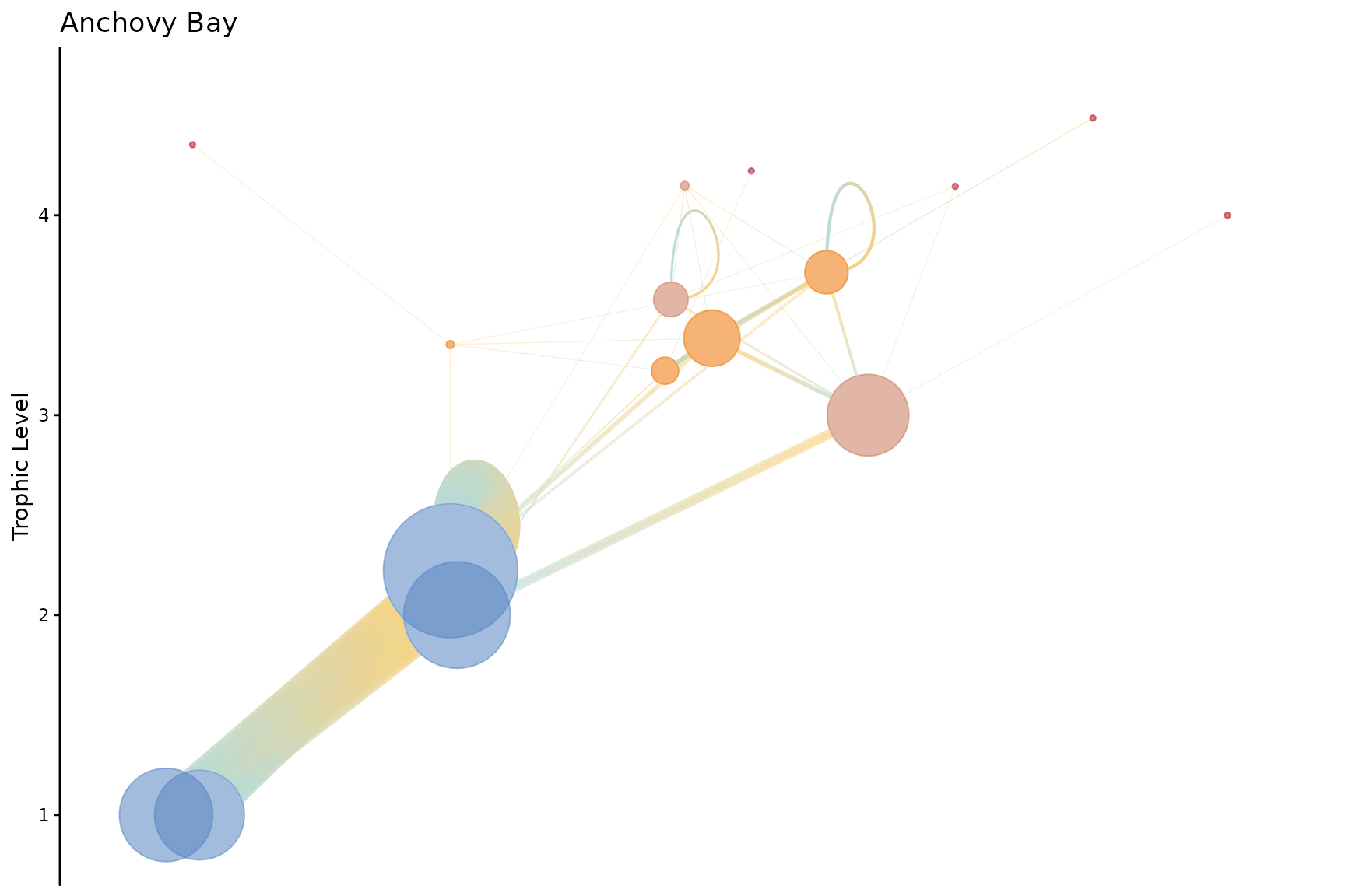

# gradient = TRUE: prey–predator colour gradient on edges
webplotviz(Rpath.obj, gradient = FALSE)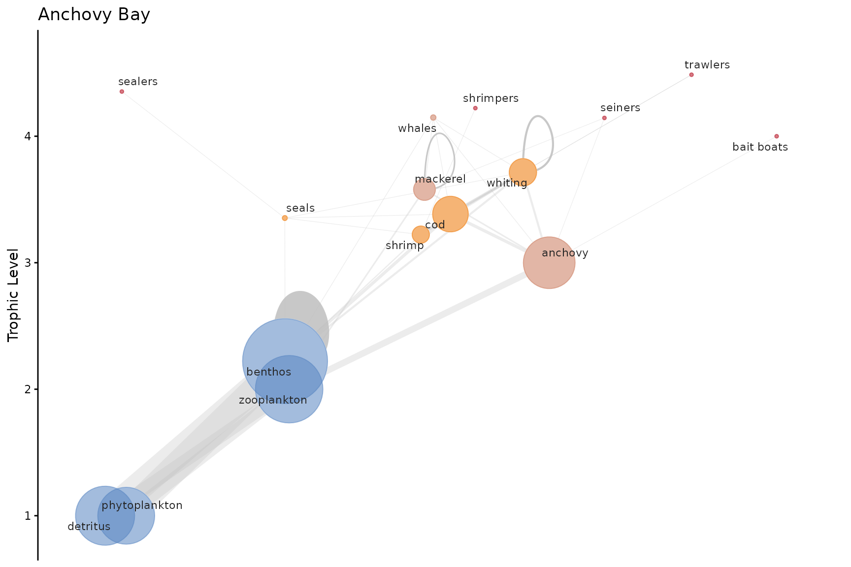

Node colouring — community detection methods

Nodes are coloured by community membership, detected with igraph’s community detection algorithms. The cluster_method parameter accepts four options:

Method	Speed	Notes
`"fast_greedy"` (default)	Fast	Good general-purpose choice for food webs
`"louvain"`	Fast	Often produces tighter communities
`"walktrap"`	Moderate	Random-walk based; works on directed graphs
`"edge_betweenness"`	Slow	Most accurate; not recommended for large webs

webplotviz(Rpath.obj, cluster_method = "fast_greedy", labels = FALSE) +
  ggplot2::ggtitle("fast_greedy (default)")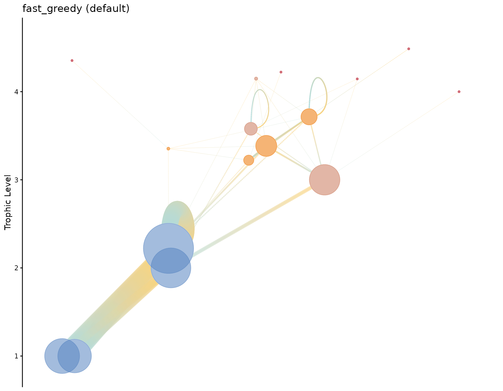

webplotviz(Rpath.obj, cluster_method = "louvain", labels = FALSE) +
  ggplot2::ggtitle("louvain")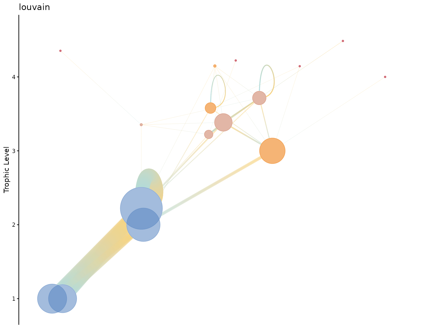

webplotviz(Rpath.obj, cluster_method = "walktrap", labels = FALSE) +
  ggplot2::ggtitle("walktrap")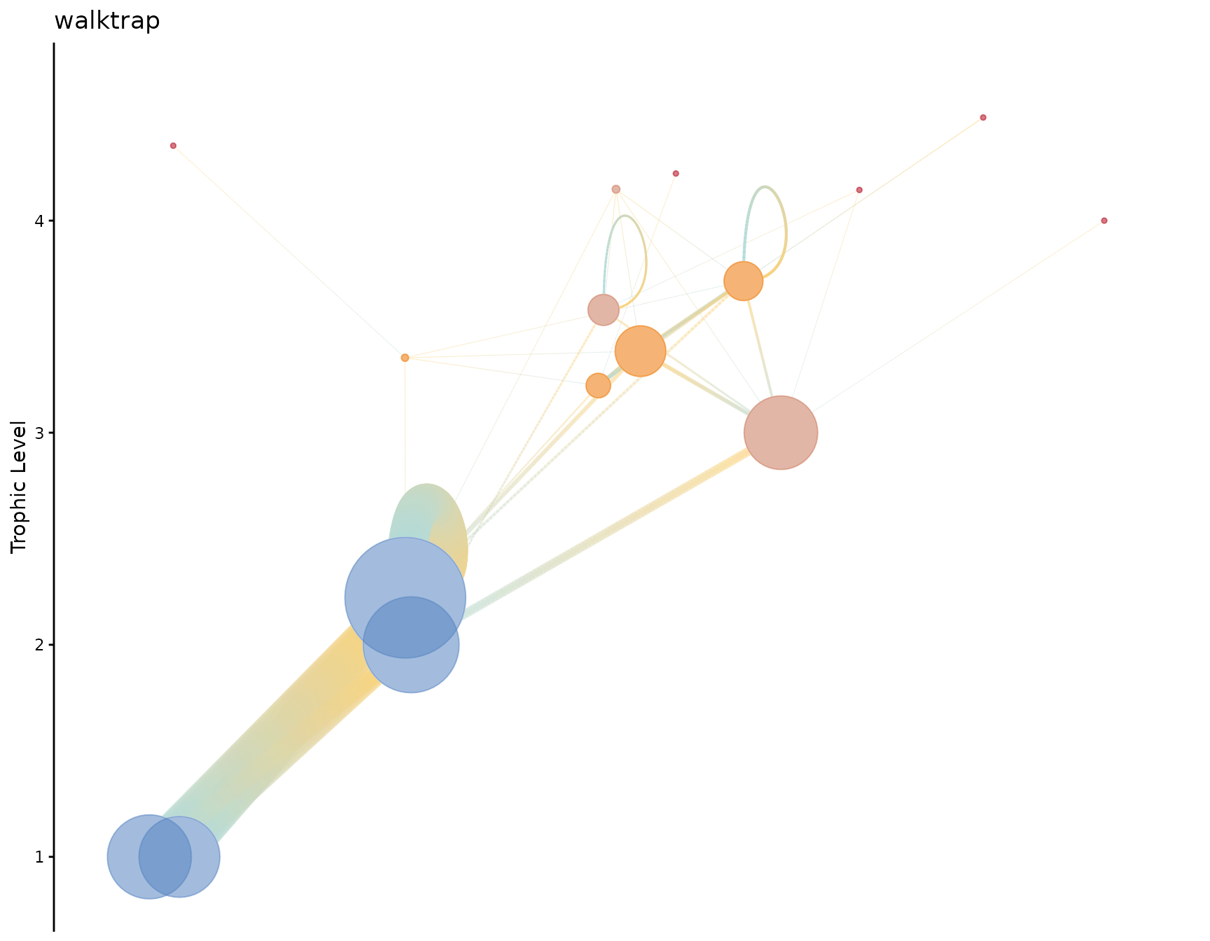

Large food web — Eastern Bering Sea

For food webs with more than 20 functional groups, plotting takes longer. The recommended workflow is to:

Use labels = FALSE to avoid the ggrepel label-placement cost.
Assign the plot to an object and save it with ggplot2::ggsave() rather than rendering it inline.

# Build the Eastern Bering Sea model
EBS.obj <- rpath(Ecosense.EBS, eco.name = "Eastern Bering Sea")

EBS.plot <- webplotviz(
  EBS.obj,
  h_spacing     = 3,
  text_size     = 2.5,
  node_size_min = 2,
  node_size_max = 30,
  labels        = FALSE
)
#> Your food web object has more than 20 functional groups.
#>     
#> Plotting to the RStudio window will take a while, please be patient...
#>     Refer to the examples for large food webs.
EBS.plot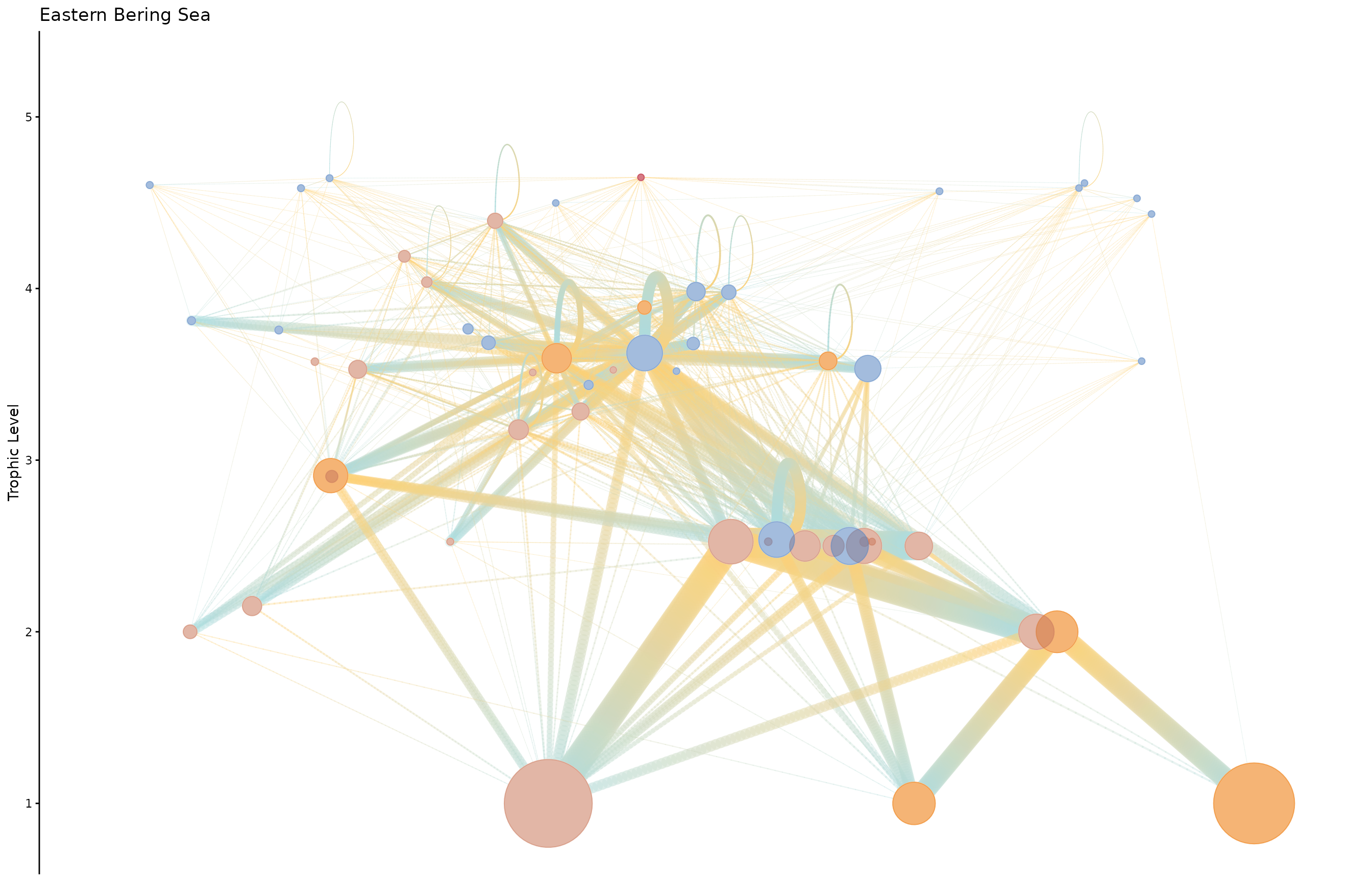

To save a high-resolution version:

ggplot2::ggsave(
  "EBS_foodweb.png",
  EBS.plot,
  width  = 16,
  height = 10,
  dpi    = 300
)